
💡 This test is performed on the Raid0 configuration and based on the formulas the IOPS and throughputs reduces 6 times on Raid6
To accurately benchmark database performance for large-scale IoT workloads, we simulated a scenario demanding approximately 170,000 data point changes per second—reflective of a typical industrial-scale environment. Using Kafka, identical message streams were fed simultaneously into MariaDB and TimeScaleDB, allowing for a direct comparison of their real-time ingest capabilities.
for i in {1..5000}; do
    ./kafka-producer-consumer -run-producer -msg-count 10000 -db mysql -dsn 'consumer:consumer@tcp(10.117.209.17:3306)/newdb' -devices-per-payload 20
    sleep 30
done
Once Kafka began generating messages, we immediately noticed increasing lag on the MariaDB side. MariaDB couldn’t ingest messages quickly enough, resulting in a steadily growing backlog. In contrast, TimeScaleDB kept pace easily, processing messages without noticeable lag. This aligns with our earlier benchmarks, where TimeScaleDB sustained a write throughput of approximately 1.4 million rows per second, compared to MariaDB’s limit of about 140,000 rows per second.
| Concurrency | Datapoints | Write Per Seconds Without Comparison | Write Per Seconds With Comparison | |
|---|---|---|---|---|
| MariaDB | 24 Partitions, 24 Consumers | 285.196.800 | 182.818 dp/s | 140.211 dp/s |
| PostgreSQL | 24 Partitions, 24 Consumers | 285.196.800 | 1.296.349 dp/s | - |
| TimescaleDB | 24 Partitions, 24 Consumers | 285.196.800 | 1.425.948 dp/s | 1.425.948 dp/s |
The graph below clearly shows how quickly TimeScaleDB ingests Kafka messages compared to MariaDB. While TimeScaleDB maintains a steady, rapid consumption rate, MariaDB experiences constant reads and steadily falls behind.
The partitioning strategy and indexing approach are identical on both MariaDB and TimeScaleDB, with each database configured to use 3-hour partitions. Both systems also utilize data compression and share the same composite index on the columns:created_dt,device_id, and metric_id.
#MariaDB Table Structure
CREATE TABLE `measurements` (
  `device_id` bigint(20) NOT NULL,
  `metric_id` bigint(20) NOT NULL,
  `value` float DEFAULT NULL,
  `created_dt` datetime DEFAULT NULL,
  KEY `created_dt_idx` (`created_dt`,`device_id`,`metric_id`)
) ENGINE=InnoDB DEFAULT CHARSET=utf8mb4 COLLATE=utf8mb4_uca1400_ai_ci ROW_FORMAT=COMPRESSED
 PARTITION BY RANGE  COLUMNS(`created_dt`)
(PARTITION `pd10` VALUES LESS THAN ('2025-03-18 00:00:00') ENGINE = InnoDB,
 PARTITION `pd11` VALUES LESS THAN ('2025-03-18 03:00:00') ENGINE = InnoDB,
 PARTITION `pd12` VALUES LESS THAN ('2025-03-18 06:00:00') ENGINE = InnoDB,
 PARTITION `pd13` VALUES LESS THAN ('2025-03-18 09:00:00') ENGINE = InnoDB,
 ...
#TimeScaleDB table structure
tscale=# \d+ measurements
Table "public.measurements"
Column | Type | Collation | Nullable | Default | Storage | Compression | Stats target | Description
------------+--------------------------+-----------+----------+---------+---------+-------------+--------------+-------------
device_id | bigint | | not null | | plain | | |
metric_id | bigint | | not null | | plain | | |
value | double precision | | | | plain | | |
created_dt | timestamp with time zone | | not null | | plain | | |
Indexes:
"ix_created_dt_metric_id" btree (created_dt, device_id, metric_id)
device_id, metric_id, value
Triggers:
ts_insert_blocker BEFORE INSERT ON measurements FOR EACH ROW EXECUTE FUNCTION _timescaledb_functions.insert_blocker()
Child tables: _timescaledb_internal._hyper_21_19717_chunk,
_timescaledb_internal._hyper_21_19718_chunk,
_timescaledb_internal._hyper_21_19719_chunk,
_timescaledb_internal._hyper_21_19720_chunk,
_timescaledb_internal._hyper_21_19721_chunk,
_timescaledb_internal._hyper_21_19722_chunk,
_timescaledb_internal._hyper_21_19723_chunk,
_timescaledb_internal._hyper_21_19724_chunk,
_timescaledb_internal._hyper_21_19725_chunk,
_timescaledb_internal._hyper_21_19726_chunk,
_timescaledb_internal._hyper_21_19727_chunk,
_timescaledb_internal._hyper_21_19729_chunk,
_timescaledb_internal._hyper_21_19731_chunk,
_timescaledb_internal._hyper_21_19733_chunk,
_timescaledb_internal._hyper_21_19735_chunk,
_timescaledb_internal._hyper_21_19747_chunk,
_timescaledb_internal._hyper_21_19748_chunk,
_timescaledb_internal._hyper_21_19749_chunk,
_timescaledb_internal._hyper_21_19750_chunk
Access method: heapThe total uncompressed dataset over a two-day period was approximately 2 TB. After enabling compression, the data size decreased to 1.6 TB on MariaDB, whereas TimeScaleDB achieved significantly better compression, reducing the data to just 158 GB.
#MariaDB partitions.
root@DB-SQL1:/var/lib/mysql/newdb# du -hs *|sort -h|tail -n5
107G	measurements#P#pd27.ibd
107G	measurements#P#pd28.ibd
109G	measurements#P#pd31.ibd
121G	measurements#P#pd17.ibd
122G	measurements#P#pd16.ibd
...


MariaDB [newdb]> select partition_name,table_rows from information_schema.partitions where table_schema='newdb' and table_name='measurements' and table_rows > 0;
+----------------+------------+
| partition_name | table_rows |
+----------------+------------+
| pd15           |  562071497 |
| pd16           | 1628687396 |
| pd17           | 1536599407 |
| pd18           | 1068136479 |
| pd21           |   34313574 |
| pd22           |    8165603 |
| pd23           |  743143627 |
| pd24           | 1640047208 |
| pd25           | 1776811458 |
| pd26           | 1792313832 |
| pd27           | 1708297643 |
| pd28           | 1748603181 |
| pd31           | 1545356537 |
| pd32           | 1809878363 |
| pd33           |  526746341 |
| pd37           |    5409840 |
| pd38           | 1081898230 |
| pd41           | 1230311361 |
| pd42           |   35063831 |
+----------------+------------+
19 rows in set (0.002 sec)
#TimeScaleDB chunk sizes
chunk_name | size_before comp. | size after comp.
-----------------------+-------------------+---------------------
_hyper_21_19717_chunk | 63 GB | 4688 MB
_hyper_21_19718_chunk | 195 GB | 14 GB
_hyper_21_19719_chunk | 198 GB | 14 GB
_hyper_21_19720_chunk | 153 GB | 11 GB
_hyper_21_19721_chunk | 8178 MB | 577 MB
_hyper_21_19722_chunk | 1821 MB | 133 MB
_hyper_21_19723_chunk | 130 GB | 9701 MB
_hyper_21_19724_chunk | 197 GB | 14 GB
_hyper_21_19725_chunk | 194 GB | 14 GB
_hyper_21_19733_chunk | 191 GB | 14 GB
_hyper_21_19726_chunk | 196 GB | 14 GB
_hyper_21_19735_chunk | 54 GB | 4018 MB
_hyper_21_19727_chunk | 193 GB | 14 GB
_hyper_21_19731_chunk | 196 GB | 14 GB
_hyper_21_19729_chunk | 197 GB | 14 GB
_hyper_21_19747_chunk | 658 MB | 53 MB
_hyper_21_19748_chunk | 121 GB | 9066 MB
_hyper_21_19749_chunk | 193 GB | 14 GB
(18 rows)
When evaluating read-query performance, we observed that MariaDB response times were notably slow—even when querying a single partition with an optimized index. In contrast, TimeScaleDB consistently returned query results within milliseconds.
We conducted tests using the following simple query, varying only the time range to measure performance:
SELECT device_id,count(1)
FROM measurements
WHERE created_dt BETWEEN '2025-03-18 16:01:16.385137+01' AND '2025-03-18 16:02:16.385137+01' and device_id IN (783,11,15)
GROUP BY device_id;
| Time Period | MariaDB | TimeScaleDB | TimeScaleDB is Faster |
|---|---|---|---|
| 1 Minutes | 26021ms | 6ms | 4,337x |
| 2 Minutes | 28231ms | 59ms | 479x |
| 5 Minutes | 2640000ms | 182ms | 14,505x |
| 10 Minutes | - | 239ms | |
| 1 Hour | - | 511ms | |
| 5 Hours | - | 1099ms |
Analysis of the execution plans confirms that queries are effectively leveraging both partition pruning and the specified composite index.
# Explain plan from MariaDB
MariaDB [newdb]> explain SELECT device_id,count(1)  FROM measurements  WHERE created_dt BETWEEN '2025-03-18 16:01:16.385137+01' AND '2025-03-18 16:02:16.385137+01' and device_id IN (783,11,15)  GROUP BY device_id \G
*************************** 1. row ***************************
           id: 1
  select_type: SIMPLE
        table: measurements
         type: range
possible_keys: created_dt_idx
          key: created_dt_idx
      key_len: 14
          ref: NULL
         rows: 25512230
        Extra: Using where; Using index; Using temporary; Using filesort
1 row in set, 2 warnings (0.001 sec)
tscale=# explain SELECT device_id,count(1)
FROM measurements
WHERE created_dt BETWEEN '2025-03-18 16:01:16.385137+01' AND '2025-03-18 16:02:16.385137+01' and device_id IN (783,11,15)
GROUP BY device_id;
                                                                                                                 QUERY PLAN
---------------------------------------------------------------------------------------------------------------------------------------------------------------------------------------------------------------------------------------------
 GroupAggregate  (cost=1.91..912.12 rows=1 width=16)
   Group Key: _hyper_21_19718_chunk.device_id
   ->  Custom Scan (DecompressChunk) on _hyper_21_19718_chunk  (cost=1.91..252.11 rows=132000 width=8)
         Vectorized Filter: ((created_dt >= '2025-03-18 16:01:16.385137+01'::timestamp with time zone) AND (created_dt <= '2025-03-18 16:02:16.385137+01'::timestamp with time zone))
         ->  Index Scan using compress_hyper_22_19730_chunk_device_id_metric_id__ts_meta__idx on compress_hyper_22_19730_chunk  (cost=0.43..252.11 rows=132 width=60)
               Index Cond: ((device_id = ANY ('{783,11,15}'::bigint[])) AND (_ts_meta_min_1 <= '2025-03-18 16:02:16.385137+01'::timestamp with time zone) AND (_ts_meta_max_1 >= '2025-03-18 16:01:16.385137+01'::timestamp with time zone))
(6 rows)

Time: 2.144 ms
We set up a Grafana dashboard to visualize data for specific devices and metrics. Queries executed against TimeScaleDB load promptly and reliably, whereas similar queries against MariaDB consistently fail or time out.
The query used to generate the Grafana visualization is as follows:
SELECT
  time_bucket('${custom_interval:text}', created_dt) AS "time",  -- Bucket the data into 1-minute intervals
  CONCAT(d.route, '.', m.name) AS series_name,
  AVG(value) AS value  -- Compute the average value for each time bucket
FROM measurements mu
JOIN metrics m ON mu.metric_id = m.id
JOIN devices d ON mu.device_id = d.id
WHERE
  $__timeFilter(created_dt) AND
  device_id IN (${Device:csv}) AND
  metric_id IN (${Metric:csv})
GROUP BY time, series_name  -- Group by time (interval) and series name
ORDER BY time, series_name;
Our detailed benchmarking clearly demonstrates the substantial advantages of migrating to TimeScaleDB for large-scale, real-time IoT workloads compared to traditional solutions like MariaDB. Here are the key insights based on rigorous testing:
Superior Write Performance
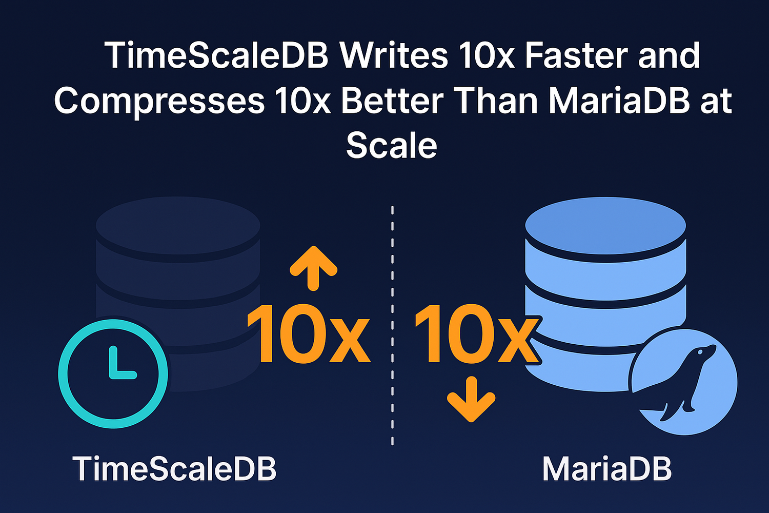
Under identical conditions, TimeScaleDB achieved a throughput of 1.4 million rows per second, whereas MariaDB maxed out at approximately 140,000 rows per second. This difference makes TimeScaleDB roughly 10 times faster at ingesting data from Kafka streams.
Massive Compression Efficiency
TimeScaleDB significantly outperformed MariaDB in data compression. Over a 2-day period, TimeScaleDB compressed 2 TB of raw data down to only 158 GB, while MariaDB managed to compress the same dataset down to just 1.6 TB. This equates to about 10x better compression, directly translating into substantial storage cost savings.
Real-time Query Performance
TimeScaleDB consistently returned query results in milliseconds, even when querying across complex, indexed partitions. In stark contrast, MariaDB exhibited poor query performance, often resulting in severe delays or outright failures during real-time dashboard usage (e.g., Grafana visualizations).
Efficient Resource Usage
Both databases utilized identical partitioning strategies (3-hour partitions) and indexing schemes (created_dt,device_id, metric_id), underscoring that the performance advantages achieved by TimeScaleDB are fundamentally due to its optimized architecture for time-series data, rather than configuration differences.
Why This Matters for Your Business
Clients relying on MariaDB or other general-purpose databases for intensive IoT, real-time monitoring, or analytical workloads risk incurring excessive infrastructure costs, poor performance, and operational bottlenecks. Moving to TimeScaleDB delivers clear benefits:
Reduced infrastructure costs due to significantly better compression and efficient use of storage resources.
Real-time responsiveness, essential for competitive advantage in rapidly evolving industrial, IoT, or analytics environments.
Future-proof scalability, easily handling billions of rows without performance degradation or complex maintenance overhead.
Don’t remain limited by your current database’s constraints. Contact us today for a personalized assessment and start leveraging the full power and efficiency of TimeScaleDB.
Thank you for reading! If you're having problems with your database, don't hesitate to contact us.
Visit our contact page.
Hinterlasse einen Kommentar
Alle Kommentare werden vor der Veröffentlichung geprüft.
Diese Website ist durch hCaptcha geschützt und es gelten die allgemeinen Geschäftsbedingungen und Datenschutzbestimmungen von hCaptcha.